k-Smooth Numbers and its Generalization
1. Introduction
A positive integer is called 


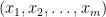
In the classic Hamming problem, we are asked to print the first 

Dijstra’s Algorithm
,
,
while
.
(
means the set
)
Putinto
endwhile


Although Dijkstra’s algorithm is designed to solve the classic Hamming problem, it is quite straightforward to extend it to solve general Hamming problem, i.e., print the first 

Let 

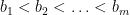


where 


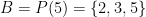
Given a smooth base 


where 

Note that 
2. Algorithm
Examinating the Dijkstra’s algorithm closely, we can see that there are two essential operations: finding the minimum of 


k-Smooth Algorithm
Initialize queues
to be empty
forfrom
to
pushinto queue
endfor
whiledo
Letand assume
forto
pushinto queue
endfor
Remove.
Put
endwhile


Theorem 1: When k-Smooth Algorithm terminates,
is the sequence of the first
generalized Hamming numbers generated by
.
To prove the theorem, we shall firstly establish two impartant facts. The first one shows that 


Fact 1: If
, then
.
Proof: We first show by induction that any element in 


Again, by induction we show that members in 


By the algorithm, we also know that elements in 


Now we have known that elements from different queues are distinct. To demonstrate that no duplicated numbers will be added to 
Before starting the next fact, we define followers of a generalized Hamming number 
Fact 2: At any time, elements in
(
) are strictly increasing and hence distinct. Also, if at step
,
is removed from some queue, then each of its
followers, either has been already pushed into some queue at some step

), or will be pushed into some queue at the step
Proof: Again, we prove it by induction. Obviously, at the very beginning of the first loop of the while block, the statement above holds. Assume the statement is correct at the step 
For 


For each 


Given these two facts established, it is quite straightforward to see the correctness of the statement in Theorem 1.
Proof: Since numbers in each queue is strictly increasing and numbers in all queues are distinct, the outputed sequence is strictly increasing and hence has no duplicates. Also, since no number will be skipped, the output sequence must contain the first
A PDF version of this article can be found here.
References
[1] Edsger W. Dijkstra. Hamming’s exercise in sasl. 1981.
An Integer Decomposition Problem
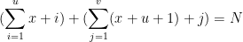
There are a lot of integer decomposition problems. Here is one of them: decompose an integer N into k different integers so that the sum of them is N and the multiplication of them is maximized. A vivid version of this problem described below.
Parliament (source: Northeastern Europe 1998): New convocation of The Fool Land’s Parliament consists of 
Input: The input file contains a single integer 
Output: Write to the output file the sizes of groups that allow the Parliament to work for the maximal possible time. These sizes should be printed on a single line in ascending order and should be separated by spaces.
Sample Input
7
Sample Output
3 4
Before introduce the solution, let us review an inequality and the multiplication principle described below.
Theorem 1 (Inequality of Arithmetric and Geometric Means) For any list of
, we have
and the equality holds if and only if
.

Theorem 2 (Multiplication Principle) If a task consists of
different operations
, and each operation
can be done by
ways. Then, there are in total
different ways to complete the task.
Back to our problem on hand. Assume that all delegates are separated into 


Unfortunately, for any 


Lemma 3 Let
when
and
are nonnegative integers and
.
has the maximal value if and only if
. Particularly, when
, the maximum of
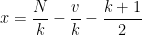
Given a increasing sequence of integers 


Lemma 4
reaches the maximal value if and only if there is at most one gap in
and that gap is at most 1 if any.
The lemma above tells us that to make 


One natural question is that, given 


Or
by assuming 


Since 


Lemma 5 Given
and
At this point, we can solve the problem as follows: For all possible 
The question following is, can we void manipulation on big integers? Yes. To make it, we need some insightful thoughts. From the example given above, it seems that 

Lemma 6 Let
Proof: We prove it by contradiction. Assume 


Now, we narrow the search scope to those
Lemma 7 Let
be the sequence maximizing
) and
starting from 3 (
), where
and
. Let
be the length of
and
. Then,
and
.
Proof: Obviously, 


Assume 


The above lemma simply states that if we get two valid sequences, namely, one starting from 2 with length 


This fact leads to following important lemma.
Lemma 8 Let valid
start from 3 (
). Then
or
.
Proof: In either case of 


Now we come to the crux of the problem. We construct a valid sequence 


array
while
end while

while
if
end if
end while


![{X[k+1] \gets k+2}](https://s0.wp.com/latex.php?latex=%7BX%5Bk%2B1%5D+%5Cgets+k%2B2%7D&bg=e7e6e2&fg=000000&s=0&c=20201002)

![{S \gets S + X[k]}](https://s0.wp.com/latex.php?latex=%7BS+%5Cgets+S+%2B+X%5Bk%5D%7D&bg=e7e6e2&fg=000000&s=0&c=20201002)


![{X[j] \gets X[j]+1}](https://s0.wp.com/latex.php?latex=%7BX%5Bj%5D+%5Cgets+X%5Bj%5D%2B1%7D&bg=e7e6e2&fg=000000&s=0&c=20201002)


The next step is to prove the algorithm is correct. Given above lemmas, it’s an easy task.
Proof: Firstly, 


The PDF version of this solution is available here.
Yet Another Note On Skewness And Kurtosis
Due to a project I recently work on, I would like to know the relationship between skewness and kurtosis. After some Google search, I am directed to Wilkins’s paper : A Note On Skewness And Kurtosis [PDF] in which he gave an new proof of the following inequality:

However, he only proved it for random variables with finite values. It’s quite natural to extend his proof to any real-valued random variable. Here is the proof I give only involving fundamental concept and definition from probability theory and quadratic form which is exactly the remarkable idea from Wilkins’s original proof.
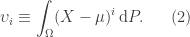
Let 


Also, denote the 

And, the standard deviation 

Define the 
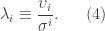
Here, 


and

Now, consider the quadratic form
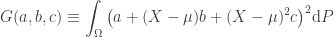

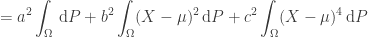


Since 


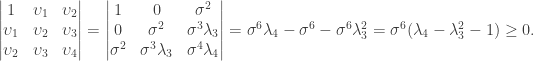
For any real-valued random variable whose standard deviation is not zero, we have

Note that standard deviation 
